 |
Hello Daniel,
Thanks again for your suggestions and hope this e-mail contributes in some sense. With our data (resting-state fMRI on mice using signals from a default mode-like networks on a fully connected 4-node model) I found that using the default
priors of spectral DCM (spm_dcm_fmri_csd.m), in many (most) subjects, the EM algorithm collapsed (around 11 iterations) into a local minima of parameters which at the end did not explain the observed variance (observed Cross-spectra). However, when using Rosa's
and Fristion's (2014, DCM for rsfMRI), I had way better estimation accuracy with >50 iterations (max. 64, changed by me). Using BMS on the BPA'd full models (all-subjects) for the three methods (default, Rosa, and Friston parameters respectively in the figure),
I found that the last set of connectivity priors (Friston's) performed better. I hope this helps... What I did was modify the spm_dcm_fmri_csd.m code after the prior selection code-line, and redefined them to the shown values in the table. However I have some
other issues that I think are very important and don't let me completely trust the results:
This is great, thanks! (Note that formally, the proper test of which priors are best is a Bayesian Model Selection to compare models with the different priors,
assuming that all the models have converged.)
1. In the models, I find some extrinsic connections to be negative (inhibitory). Physiologically speaking this should not happen as long-range connections in general are excitatory. I will eventually try more complicated models with P-DCM
(Havlicek et. al, 2015), but standard DCM should be enough at least to have a model structure that does not violate observed long-range causal effects.
Remember that DCM isn’t modelling axons – it’s representing causal influence. So a long-range excitatory connection could excite local inhibition in the target
region, and have an overall inhibitory effect. You could, however, switch on the 2-state DCM option (Marreiros et al. 2008 – documentation at
https://en.wikibooks.org/wiki/SPM/Two_State_DCM ). This enforces excitatory long-range connections and local inhibition.
2. Regarding the hemodynamic parameters. I will also try to modify the values (priors on epsilon) with our scanner strength (7 Tesla), but regarding the hemodynamic state parameters (transit, and decay) I have found that in some subjects
I obtain a negative value for transit time, which should not happen (negative time). You recommended me to start with these found posteriors as priors, but I can't use a negative transit time (I am also putting an image of the found parameter posteriors for
reference). Once again, this is resting-state modelling we are talking about and the proposed hemodynamic model proposed may differ under these circumstances. My question would if you would recommend allowing all parameters of the model to be free and/or use
a simpler network (say 2-nodes with know directional structural connectivity) and investigate the effect of the hemodynamic parameters?
Transit and decay are log parameters – so you need to do exp(transit) to get the proper value :-) The thing to watch out for is posterior covariance between neuronal
and haemodynamic parameters. Take a look at the Cp matrix – let me know if you need help with that. If you’re interested in haemodynamics, and they covary highly with the neuronal parameters, it may be worth having a simpler model.
3. Finally, is there any recommendation on how I can "force" the EM algorithm in spm_nlsi_GN.m to do at least a certain amount of iterations until an acceptable amount of variance is explained by the inverted model?
This function will iterate until the free energy stops improving, or the M.Nmax (=128) is hit. If you have difficulty with lack of convergence, the problem isn’t
the maximum number of iterations, but rather something up with the model.
Best,
Peter
I appreciate your (and the community's) help here and hope these issues with resting-state modelling can be jointly resolved.
Best regards,
Fig. 1. Proposed priors on expectations (pE) and covariances pC: 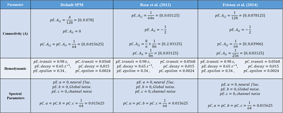
Fig. 2. Found posteriors: 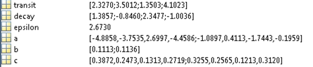
Daniel Gutierrez Barragan, PhD Student
Center for Neuroscience and Cognitive Systems (CIMeC)
Italian Institute of Technology (IIT)
University of Trento
Rovereto (TN): Palazzo Fedrigotti - corso Bettini 31
2015-08-21 12:20 GMT+02:00 Zeidman, Peter <[log in to unmask]>:
Dear Daniel,
This project sounds very impressive. I will address what I can – one answer I will need to confirm when my colleagues return from holiday in September.
I am working with resting state fMRI data acquired from rodents, have built a function to specify a DCM.mat structure with all the data necesary, and have run full and selected models for the Default Mode Network (DMN), extracting signals from preprocessed data for 4 ROIs. I am using spectral and stochastic DCM (from my own function, not using the GUI) for comparison but have a couple of questions ( in advance I apologize for the length of this, and the over-description, but I mean to be very specific):
1. Free-Energy (F). F is supposed to be a bound on the log(evidence), and being the evidence a probability this log(evidence) should be negative (0, -Inf). Hoewever, for some subjects and models I get positive F and for others Negative (even with the same model). According to the Variational Laplace approach this should not happen right? Also, it seems that F is very similar for every model family for a single subjects, but varies a lot between them for the same model. What values of F are acceptable and will post-hoc optimization correct this?
Absolute values of the free energy are arbitrary and are always used as a relative measure, compared to some other model. (In the case of estimating models, the value of F calculated on each iteration of the EM algorithm relative to the previous iteration, and the sign is irrelevant.)
So what counts is the difference between the (log) free energy of two models – known as the (log) Bayes factor, i.e.
logBF = DCM1.F – DCM2.F;
This quantifies how much better one model is than another, in terms of accuracy and complexity. A log Bayes factor or 3 equates to 95% confidence that one model is better than another. At the group level, there are fixed effects and random effects methods for summarising these free energies across subjects, which you can access using the SPM GUI.
2. Variance Explained. Using spm_dcm_fmri_check.m I checked for the variance each model (per subject) explained and Free-Energy does not seem to play a role in this calculation. This explained variance is a measure of the model fit, but I assume it does not account for model complexity. In this sense, how can I check that a model is well balanced in terms of accuracy and complexity with the DCM results file?
You are entirely correct that explained variance doesn’t penalise complexity, and is only a sanity check to ensure that a reasonable amount of the signal is being explained. The measure of whether accuracy and complexity are well balanced is the free energy (DCM.F), which can be thought of as accuracy minus complexity. As I mentioned, this will always be relative to some other model.
3. Post-hoc. For the full model case, should I do post-hoc optimization for each subject and then Bayesian Parameter Averaging (BPA)? Or should I just run a joint (all subjects included) post-hoc analysis? I am trying to follow the methods used in Razi et al "Construct validation of a DCM for resting state fMRI" and this is not very clear to me.
I suggest you put in all your subjects, and the script will try to find an optimal model at the group level. It will also generate a BPA.mat file, in the folder of the first subject.
4.Options. The "DCM.options" structure is particularly broad in terms of the information it contains. However, when defining the priors in spm_dcm_fmri_priors.m there are two values I don't completely understand which completely define the priors for the Effective Connectivity (EC) matrix, "pA" and "dA" namely precision and decay of connections. These values are described in Friston et al. original DCM paper "Dynamic Causal Modelling" as and in the priors program are set (for one hidden state per node) by default to pA = 64, and dA = 1. Is there a specific reason for these values?
To be confirmed.
5. Hemodynamic Priors. After the paper Stephan et al. "Comparing Hemodynamic Models with DCM", SPM uses the function spm_fx_fmri.m to compute the states (dynamic equation and hemodynamic equations) of the system, and spm_gx_fmri.m computes the corresponding modelled BOLD response. spm_fx fixes the hemodynamic parameters (vector H) corresponding to autoregulation (kappa); rate of elimination (gamma); grubb's exponent (alpha); and resting Ox. extraction (E0 or rho. It also leaves signal decay and transit time as free parameters. spm_gx on ly has as free parameter epsilon, as described in the mentioned paper. After performing spectral and stochastic DCM for resting state data, these parameters vary a lot between subjects and models. I was wondering if there is any recommendations for mice data and/or resting-state fMRI?
When this has previously come up in discussion, the feeling has been that haemodynamic parameters should be similar across mammalian species. To develop a custom prior for epsilon, you could perform a DCM analysis on a group of mice, average the posterior estimate for epsilon across subjects, and then use this estimate as the new prior - either to re-estimate all the existing models to finesse the models, or use this for subsequent experiments with independent mice. I’m not aware of any specific haemodynamic issues for resting state data, although resting state is not my area of expertise.
Also, there are some differences between how SPM12 by default sets priors. Since Stephan et al. these priors are set, however, subsequent papers such as Rosa et al. "Post-hoc optimization of DCMs" (appendix A); and Friston et al. "A DCM for resting state fMRI" have different ways of calculating them.
The priors do get improved from time to time – I’d recommend using the latest version of SPM / DCM, and stick with the same version throughout your analysis.
6. Connectivity Priors. I inverted full and selected models for the DMN (4nodes) using spectral DCM with default priors; by modifying them according to Rosa et al.(post-hoc...); and then modifying them according to Friston et al. (DCM for rsfMRI). Default prior estimation yields shrinked (=0) intrinsic connections and 1/128 extrinsic, corresponding to slow modes in the system. Rosa et al. propose parameters priors based on the amount of nodes: A intrinsic = -1/2 with variance 1/8n, and A-extrinsic = 1/64n with variance (8/n) + (1/8n = 2.03. Finally, Friston et al. propose A-intrinsic = -1/2 with variance 1/256, and A-extrinsic = 1/128 with variance 1/64. After inverting models for many subjects, I saw that modifying these priors yielded models with different (even oposite sign) Free-Energies and much more accurate models with explained variances of over 50% and even some reaching 90% (oh, and with even less EM-algorithm iterations). This Compared to the default prior values, in which many models for the same subjects could not explain more than 10% variance. Are there any recommendations on which approach to use? For mice?
You have posed a very nice model comparison question – does one set of priors do better or worse than another set of priors? As you said yourself, you can’t compare models based on the explained variance – the complexity won’t be matched. Instead, I suggest you first estimate models with each set of priors. Then, put all the models into Bayesian Model Selection (click ‘Dynamic Causal Modelling’, then ‘Compare’). Use this screen to define two ‘families’ of models – each with a different set of priors. You will then get the posterior probability for each family (each set of priors) – based on the free energy.
Feel free to ask any further questions.
Best,
Peter