That's really interesting! Since the fits then and now were both
least-squares, I wonder how Cromer & Mann could have gotten it so far
off? Looking at the residuals, I see that although that of nitrogen
oscillates badly, even the worst outlier is still within 0.01 electrons
of the Hartree-Fock values. Perhaps 1% of an electron was their
convergence limit?
Either way, I think it would be valuable to have a "re-fit" of the Table
6.1.1.1/3 values without the "c" term. Then we can go all the way to
B=0 without worrying about singularities.
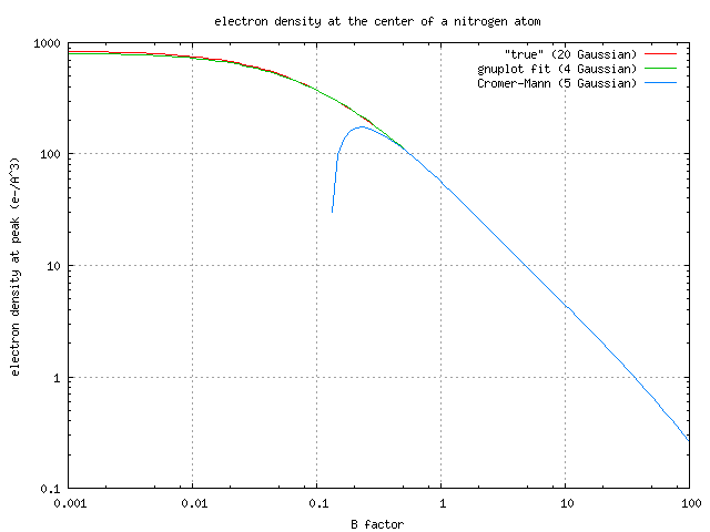
For example, I attach here a plot of the electron density at the center
of a nitrogen atom vs B factor (in real space). The red curve is the
result of a 20-Gaussian fit to the data for nitrogen in table 6.1.1.1
all the way out to sin(theta)/lambda = 6 (although 7 Gaussians is more
than enough). This "true" curve approaches 1000 e-/A^3 as B approaches
zero, but the 5-Gaussian model using the Cromer-Mann coefficients form
6.1.1.4 (blue curve) starts to deviate when B becomes less than one, and
actually goes negative for B < 0.1. A simpler model (without the c
term, but re-fit) is the green line. Very much like what Tim suggested.
Not exactly a problem for typical macromolecular refinement, but
still... I wonder what would happen if I edited my ${CLIBD}/atomsf.lib ?
-James Holton
MAD Scientist
On 9/18/2012 6:32 AM, Tim Gruene wrote:
> -----BEGIN PGP SIGNED MESSAGE-----
> Hash: SHA1
>
> Hello Oliver,
>
> when you fit the values from ICA Tab 6.1.1.1 with gnuplot, the values
> of C and N become much more comparable. c(C) = 0.017 and especially
> c(N) = 0.025 > 0!!!
> for C:
> Final set of parameters Asymptotic Standard Error
> ======================= ==========================
>
> a1 = 0.604126 +/- 0.02326 (3.85%)
> a2 = 2.63343 +/- 0.03321 (1.261%)
> a3 = 1.52123 +/- 0.03528 (2.319%)
> a4 = 1.2211 +/- 0.02225 (1.822%)
> b1 = 0.185807 +/- 0.00629 (3.385%)
> b2 = 14.6332 +/- 0.1355 (0.9263%)
> b3 = 41.6948 +/- 0.5345 (1.282%)
> b4 = 0.717984 +/- 0.01251 (1.743%)
> c = 0.0171359 +/- 0.002045 (11.93%)
>
> for N:
> Final set of parameters Asymptotic Standard Error
> ======================= ==========================
>
> a1 = 0.723788 +/- 0.04334 (5.988%)
> a2 = 3.24589 +/- 0.04074 (1.255%)
> a3 = 1.90049 +/- 0.04422 (2.327%)
> a4 = 1.10071 +/- 0.0413 (3.752%)
> b1 = 0.157345 +/- 0.007552 (4.8%)
> b2 = 10.106 +/- 0.1041 (1.03%)
> b3 = 30.0211 +/- 0.3946 (1.314%)
> b4 = 0.567116 +/- 0.01914 (3.376%)
> c = 0.0252303 +/- 0.003284 (13.01%)
>
> In 1967, Mann only calculated to sin \theta/lambda = 0, ... 1.5, and
> their tabulated values do indeed fit decently within that range, but
> not out to 6A.
>
> I thought this was notworthy, and I am curious which values for these
> constants refinement programs use nowadays. Maybe George, Garib,
> Pavel, and Gerard may want to comment?
>
> Cheers,
> Tim
>
> On 09/18/2012 10:11 AM, Oliver Einsle wrote:
>> Hi there,
>>
>> I was just pointed to this thread and should comment on the
>> discussion, as actually made the plots for this paper. James has
>> clarified the issue much better than I could have, and indeed the
>> calculations will fail for larger Bragg angles if you do not assume
>> a reasonable B-factor (I used B=10 for the plots).
>>
>> Doug Rees has pointed out at the time that for large theta the
>> c-term of the Cromer/Mann approximation becomes dominant, and this
>> is where chaos comes in, as the Cromer/Mann parameters are only
>> derived from a fit to the actual HF-calculation. They are numbers
>> without physical meaning, which becomes particularly obvious if you
>> compare the parameters for C and N:
>>
>>
>> C: 2.3100 20.8439 1.0200 10.2075 1.5886 0.5687 0.8650
>> 51.6512 0.2156 N: 12.2126 0.0057 3.1322 9.8933 2.0125
>> 28.9975 1.1663 0.5826 -11.5290
>>
>> The scattering factors for these are reasonably similar, but the
>> c-values are entirely different. The B-factor dampens this out and
>> this is an essential point.
>>
>>
>>
>> For clarity: I made the plots using Waterloo Maple with the
>> following code:
>>
>> restart; SF :=Matrix(17,9,readdata("scatter.dat",float,9));
>>
>> biso := 10; e := 1; AFF :=
>> (e)->(SF[e,1]*exp(-SF[e,2]*s^2)+SF[e,3]*exp(-SF[e,4]*s^2)
>> +SF[e,5]*exp(-SF[e,6]*s^2)+SF[e,7]*exp(-SF[e,8]*s^2)
>> +SF[e,9])*exp(-biso*s^2/4);
>>
>> H := AFF(1); C := AFF(2); N := AFF(3); Ox :=
>> AFF(4); S := AFF(5); Fe := AFF(6); Fe2 := AFF(7); Fe3 :=
>> AFF(8); Cu := AFF(9); Cu1 := AFF(10); Cu2 := AFF(11); Mo
>> := AFF(12); Mo4 := AFF(13); Mo5 := AFF(14); Mo6 := AFF(15);
>>
>> // Plot scattering factors
>>
>> plot([C,N,Fe,S], s=0..1);
>>
>>
>> // Figure 1:
>>
>> rho0 := (r) -> Int((4*Pi*s^2)*Fe2*sin(2*Pi*s*r)/(2*Pi*s*r),
>> s=0..1/dmax); dmax := 1.0; plot (rho0, -5..5);
>>
>>
>> // Figure 1 (inset): Electron Density Profile
>>
>> rho := (r,f)
>> ->(Int((4*Pi*s^2)*f*sin(2*Pi*s*r)/(2*Pi*s*r),s=0..1/dmax));
>> cofactor:= 9*rho(3.3,S) + 6*rho(2.0,Fe2) + 1*rho(3.49,Mo6) +
>> 1*rho(3.51,Fe3); plot(cofactor, dmax=0.5..3.5);
>>
>>
>> The file scatter.dat is simply a collection of some form factors,
>> courtesy of atomsf.lib (see attachment).
>>
>>
>>
>> Cheers,
>>
>> Oliver.
>>
>>
>>
>> Am 9/17/12 11:24 AM schrieb "Tim Gruene" unter
>> <[log in to unmask]>:
>>
>> Dear James et al.,
>>
>> so to summarise, the answer to Niu's question is that he must add
>> a factor of e^(-Bs^2) to the formula of Cromer/Mann and then adjust
>> the value of B until it matches the inset. Given that you claim
>> rho=0.025e/A^3 (I assume for 1/dmax approx. 0) for B=12 and the
>> inset shows a value of about 0.6, a somewhat higher B-value should
>> work.
>>
>> Cheers, Tim
>>
>> On 09/17/2012 08:32 AM, James Holton wrote:
>>>>> Yes, the constant term in the "5-Gaussian" structure factor
>>>>> tables does become annoying when you try to plot electron
>>>>> density in real space, but only if you try to make the B
>>>>> factor zero. If the B factors are ~12 (like they are in
>>>>> 1m1n), then the electron density 2.0 A from an Fe atom is not
>>>>> -0.2 e-/A^3, it is 0.025 e-/A^3. This is only 1% of the
>>>>> electron density at the center of a nitrogen atom with the
>>>>> same B factor.
>>>>>
>>>>> But if you do set the B factor to zero, then the electron
>>>>> density at the center of any atom (using the 5-Gaussian
>>>>> model) is infinity. To put it in gnuplot-ish, the structure
>>>>> factor of Fe (in reciprocal space) can be plotted with this
>>>>> function:
>>>>>
>>>>> Fe_sf(s)=Fe_a1*exp(-Fe_b1*s*s)+Fe_a2*exp(-Fe_b2*s*s)+Fe_a3*exp(-Fe_b3*s*s
>>>>>
>>>>>
> )+Fe_a4*exp(-Fe_b4*s*s)+Fe_c
>>>>>
>>>>> where: Fe_c = 1.036900; Fe_a1 = 11.769500; Fe_a2 = 7.357300;
>>>>> Fe_a3 = 3.522200; Fe_a4 = 2.304500; Fe_b1 = 4.761100; Fe_b2 =
>>>>> 0.307200; Fe_b3 = 15.353500; Fe_b4 = 76.880501; and "s" is
>>>>> sin(theta)/lambda
>>>>>
>>>>> applying a B factor is then just multiplication by
>>>>> exp(-B*s*s)
>>>>>
>>>>>
>>>>> Since the terms are all Gaussians, the inverse Fourier
>>>>> transform can actually be done analytically, giving the
>>>>> real-space version, or the expression for electron density vs
>>>>> distance from the nucleus (r):
>>>>>
>>>>> Fe_ff(r,B) = \
>>>>> +Fe_a1*(4*pi/(Fe_b1+B))**1.5*safexp(-4*pi**2/(Fe_b1+B)*r*r)
>>>>> \ +Fe_a2*(4*pi/(Fe_b2+B))**1.5*safexp(-4*pi**2/(Fe_b2+B)*r*r)
>>>>> \ +Fe_a3*(4*pi/(Fe_b3+B))**1.5*safexp(-4*pi**2/(Fe_b3+B)*r*r)
>>>>> \ +Fe_a4*(4*pi/(Fe_b4+B))**1.5*safexp(-4*pi**2/(Fe_b4+B)*r*r)
>>>>> \ +Fe_c *(4*pi/(B))**1.5*safexp(-4*pi**2/(B)*r*r);
>>>>>
>>>>> Where here applying a B factor requires folding it into each
>>>>> Gaussian term. Notice how the Fe_c term blows up as B->0?
>>>>> This is where most of the series-termination effects come
>>>>> from. If you want the above equations for other atoms, you
>>>>> can get them from here:
>>>>> http://bl831.als.lbl.gov/~jamesh/pickup/all_atomsf.gnuplot
>>>>> http://bl831.als.lbl.gov/~jamesh/pickup/all_atomff.gnuplot
>>>>>
>>>>> This "infinitely sharp spike problem" seems to have led some
>>>>> people to conclude that a zero B factor is non-physical, but
>>>>> nothing could be further from the truth! The scattering from
>>>>> mono-atomic gasses is an excellent example of how one can
>>>>> observe the B=0 structure factor. In fact, gas scattering
>>>>> is how the quantum mechanical self-consistent field
>>>>> calculations of electron clouds around atoms was
>>>>> experimentally verified. Does this mean that there really is
>>>>> an infinitely sharp "spike" in the middle of every atom? Of
>>>>> course not. But there is a "very" sharp spike.
>>>>>
>>>>> So, the problem of "infinite density" at the nucleus is
>>>>> really just an artifact of the 5-Gaussian formalism.
>>>>> Strictly speaking, the "5-Gaussian" structure factor
>>>>> representation you find in ${CLIBD}/atomsf.lib (or Table
>>>>> 6.1.1.4 in the International Tables volume C) is nothing more
>>>>> than a curve fit to the "true" values listed in ITC volume C
>>>>> tables 6.1.1.1 (neutral atoms) and 6.1.1.3 (ions). These
>>>>> latter tables are the Fourier transform of the "true"
>>>>> electron density distribution around a particular atom/ion
>>>>> obtained from quantum mechanical self-consistent field
>>>>> calculations (like those of Cromer, Mann and many others).
>>>>>
>>>>> The important thing to realize is that the fit was done in
>>>>> _reciprocal_ space, and if you look carefully at tables
>>>>> 6.1.1.1 and 6.1.1.3, you can see that even at REALLY high
>>>>> angle (sin(theta)/lambda = 6, or 0.083 A resolution) there is
>>>>> still significant elastic scattering from the heavier atoms.
>>>>> The purpose of the "constant term" in the 5-Gaussian
>>>>> representation is to try and capture this high-angle "tail",
>>>>> and for the really heavy atoms this can be more than 5
>>>>> electron equivalents. In real space, this is equivalent to
>>>>> saying that about 5 electrons are located within at least
>>>>> ~0.03 A of the nucleus. That's a very short distance, but it
>>>>> is also not zero. This is because the first few shells of
>>>>> electrons around things like a Uranium nucleus actually are
>>>>> very small and dense. How, then, can we have any hope of
>>>>> modelling heavy atoms properly without using a map grid
>>>>> sampling of 0.01A ? Easy! The B factors are never zero.
>>>>>
>>>>> Even for a truly infinitely sharp peak (aka a single
>>>>> electron), it doesn't take much of a B factor to spread it
>>>>> out to a reasonable size. For example, applying a B factor of
>>>>> 9 to a point charge will give it a full-width-half max (FWHM)
>>>>> of 0.8 A, the same as the "diameter" of a carbon atom. A
>>>>> carbon atom with B=12 has FWHM = 1.1 A, the same as a "point"
>>>>> charge with B=16. Carbon at B=80 and a point with B=93 both
>>>>> have FWHM = 2.6 A. As the B factor becomes larger and
>>>>> larger, it tends to dominate the atomic shape (looks like a
>>>>> single Gaussian). This is why it is so hard to assign atom
>>>>> types from density alone. In fact, with B=80, a Uranium atom
>>>>> at 1/100th occupancy is essentially indistinguishable from a
>>>>> hydrogen atom. That is, even a modest B factor pretty much
>>>>> "washes out" any sharp features the atoms might have.
>>>>> Sometimes I wonder why we bother with "form factors" at all,
>>>>> since at modest resolutions all we really need is Z (the
>>>>> atomic number) and the B factor. But, then again, I suppose
>>>>> it doesn't hurt either.
>>>>>
>>>>>
>>>>> So, what does this have to do with series termination?
>>>>> Series termination arises in the inverse Fourier transform
>>>>> (making a map from structure factors). Technically, the
>>>>> "tails" of a Gaussian never reach zero, so any sort of
>>>>> "resolution cutoff" always introduces some error into the
>>>>> electron density calculation. That is, if you create an
>>>>> arbitrary electron-density map, convert it into structure
>>>>> factors and then "fft" it back, you do _not_ get the same map
>>>>> that you started with! How much do they differ? Depends on
>>>>> the RMS value of the high-angle structure factors that have
>>>>> been cut off (Parseval's theorem). The "infinitely sharp
>>>>> spike" problem exacerbates this, because the B=0 structure
>>>>> factors do not tend toward zero as fast as a Gaussian with
>>>>> the "atomic width" would.
>>>>>
>>>>> So, for a given resolution, when does the B factor get "too
>>>>> sharp"? Well, for "protein" atoms, the following B factors
>>>>> will introduce an rms error in the electron density map equal
>>>>> to about 5% of the peak height of the atoms when the data are
>>>>> cut to the following resolution: d B 1.0 <5 1.5 8 2.0 27
>>>>> 2.5 45 3.0 65 3.5 86 4.0 >99
>>>>>
>>>>> smaller B factors than this will introduce more than 5% error
>>>>> at each of these resolutions. Now, of course, one is often
>>>>> not nearly as concerned with the average error in the map as
>>>>> you are with the error at a particular point of interest, but
>>>>> the above numbers can serve as a rough guide. If you want to
>>>>> see the series-termination error at a particular point in the
>>>>> map, you will have to calculate the "true" map of your model
>>>>> (using a program like SFALL), and then run the map back and
>>>>> forth through the Fourier transform and resolution cutoff
>>>>> (such as with SFALL and FFT). You can then use MAPMAN or
>>>>> Chimera to probe the electron density at the point of
>>>>> interest.
>>>>>
>>>>> But, to answer the OP's question, I would not recommend
>>>>> trying to do fancy map interpretation to identify a mystery
>>>>> atom. Instead, just refine the occupancy of the mystery atom
>>>>> and see where that goes. Perhaps jiggling the rest of the
>>>>> molecule with "kick maps" to see how stable the occupancy is.
>>>>> Since refinement only does forward-FFTs, it is formally
>>>>> insensitive to series termination errors. It is only map
>>>>> calculation where series termination can become a problem.
>>>>>
>>>>> Thanks to Garib for clearing up that last point for me!
>>>>>
>>>>> -James Holton MAD Scientist
>>>>>
>>>>>
>>>>> On 9/15/2012 3:12 AM, Tim Gruene wrote: Dear Ian,
>>>>>
>>>>> provided that f(s) is given by the formula in the Cromer/Mann
>>>>> article, which I believe we have agreed on, the inset of
>>>>> Fig.1 of the Science article we are talking about is claimed
>>>>> to be the graph of the function g, which I added as pdf to
>>>>> this email for better readability.
>>>>>
>>>>> Irrespective of what has been plotted in any other article
>>>>> meantioned throughout this thread, this claim is incorrect,
>>>>> given a_i, b_i, c > 0.
>>>>>
>>>>> I am sure you can figure this out yourself. My argument was
>>>>> not involving mathematical programs but only one-dimensional
>>>>> calculus.
>>>>>
>>>>> Cheers, Tim
>>>>>
>>>>> On 09/14/2012 04:46 PM, Ian Tickle wrote:
>>>>>>>> On 14 September 2012 15:15, Tim Gruene
>>>>>>>> <[log in to unmask]> wrote:
>>>>>>>>> -----BEGIN PGP SIGNED MESSAGE----- Hash: SHA1
>>>>>>>>>
>>>>>>>>> Hello Ian,
>>>>>>>>>
>>>>>>>>> your article describes f(s) as sum of four Gaussians,
>>>>>>>>> which is not the same f(s) from Cromer's and Mann's
>>>>>>>>> paper and the one used both by Niu and me. Here, f(s)
>>>>>>>>> contains a constant, as I pointed out to in my
>>>>>>>>> response, which makes the integral oscillate between
>>>>>>>>> plus and minus infinity as the upper integral border
>>>>>>>>> (called 1/dmax in the article Niu refers to) goes to
>>>>>>>>> infinity).
>>>>>>>>>
>>>>>>>>> Maybe you can shed some light on why your article
>>>>>>>>> uses a different f(s) than Cromer/Mann. This
>>>>>>>>> explanation might be the answer to Nius question, I
>>>>>>>>> reckon, and feed my curiosity, too.
>>>>>>>> Tim & Niu, oops yes a small slip in the paper there, it
>>>>>>>> should have read "4 Gaussians + constant term": this is
>>>>>>>> clear from the ITC reference given and the
>>>>>>>> $CLIBD/atomsf.lib table referred to. In practice it's
>>>>>>>> actually rendered as a sum of 5 Gaussians after you
>>>>>>>> multiply the f(s) and atomic Biso factor terms, so
>>>>>>>> unless Biso = 0 (very unphysical!) there is actually no
>>>>>>>> constant term. My integral for rho(r) certainly
>>>>>>>> doesn't oscillate between plus and minus infinity as
>>>>>>>> d_min -> zero. If yours does then I suspect that
>>>>>>>> either the Biso term was forgotten or if not then a bug
>>>>>>>> in the integration routine (e.g. can it handle properly
>>>>>>>> the point at r = 0 where the standard formula for the
>>>>>>>> density gives 0/0?). I used QUADPACK
>>>>>>>> (http://people.sc.fsu.edu/~jburkardt/f_src/quadpack/quadpack.html)
>>>>>>>>
>>>>>>>>
> which seems pretty good at taking care of such singularities
>>>>>>>> (assuming of course that the integral does actually
>>>>>>>> converge).
>>>>>>>>
>>>>>>>> Cheers
>>>>>>>>
>>>>>>>> -- Ian
>>>>>>>>
>>>>> -- - -- Dr Tim Gruene Institut fuer anorganische Chemie
>>>>> Tammannstr. 4 D-37077 Goettingen
>>>>>
>>>>> GPG Key ID = A46BEE1A
>>>>>
>>>>>
> - --
> - --
> Dr Tim Gruene
> Institut fuer anorganische Chemie
> Tammannstr. 4
> D-37077 Goettingen
>
> GPG Key ID = A46BEE1A
>
> -----BEGIN PGP SIGNATURE-----
> Version: GnuPG v1.4.12 (GNU/Linux)
> Comment: Using GnuPG with Mozilla - http://enigmail.mozdev.org/
>
> iD8DBQFQWHfUUxlJ7aRr7hoRAr4VAJ4isN0PLYafsdZgVOYseV+MricBVgCfftQd
> 4a7EpBF1hud6sM6L0SxBXqE=
> =ijgy
> -----END PGP SIGNATURE-----
|


